I’ve always struggled to understand the intuitions behind Fully Sharded Data Parallel beyond the high level idea of “shard everything.” Without a systems background, the fundamental primitives like “all-reduce” and “reduce-scatter” aren’t in my vocabulary. But FSDP conceptually is not complicated, especially once you state what the goals are (the rest is nearly necessitated by the engineering).
This post is an attempt to deconstruct the algorithm from first principles as a non-systems person. I will bring up the primitives in their specified context, which I think helps reinforces the intuition much better. Most ML researchers have a stronger understanding of the models, params, and optimizer processes than the systems jargon anyways.
Thanks to Gemini and Tim Darcet’s off-hand comment about FSDP for clarifying my intuitions [1].
How to Train your Machine Learning Model
How does one train a machine learning model? In the simplest case, such as doing a Coursera Intro to Machine Learning course, you’ll be training on your personal laptop, which likely only has a CPU. This will be very slow, as CPUs aren’t optimized for computing, but at least you’re training a model and doing machine learning!
What is the limiting factor here? You’re capped by your CPU’s memory, i.e. the Random Access Memory (RAM). For example, my Macbook Pro has 32GB of Unified Memory. Quite the uphill battle here, since Google Chrome has likely already consumed most of it!
You’ll need to store almost everything in RAM for training to not be prohibitively slower than it already is. This includes
- the dataset, which can be 200MB if you’re using CIFAR-10, 150GB if you’re using ImageNet, or 5TB+ for LLM pretraining sets like RedPajama (if loaded in memory).
- the model weights, i.e. the model itself.
- the model activations, for computing the gradients later on.
- the model gradients (and optimizer states), for updating the model with backpropagation.
Every systems optimization which makes training faster and less memory-intensive revolves around trading off and improving these factors.
Now in practice, to get anywhere with machine learning, you’ll need a hardware accelerator. So let’s say we were graciously gifted a single GPU for Christmas, which we’ll use to speed up our training. GPUs are good for one thing: speeding up matrix multiplications.
That’s handy, as those are most of our model’s computations. However, if we want to take advantage of these speedups, we’ll need to move our data and model to the GPU, which is dependent on the CPU<->GPU transfer time, otherwise known as the PCIe bandwidth. For the L40 GPUs that I generally use, Gemini tells me that they support PCIe 4.0 with a bandwidth of 64 GB/s bi-directional, so moving a a 10GB dataset from system RAM onto the GPU should take ~0.2s.
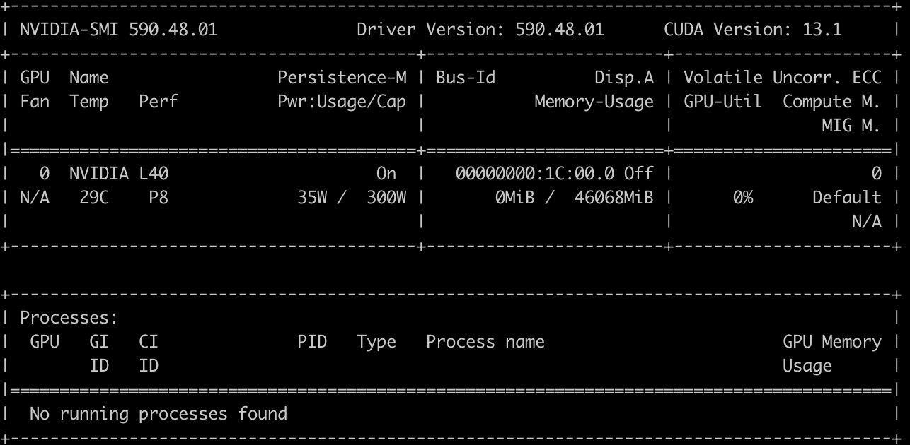
nvidia-smi output for a 1-GPU instance
For a long time in computer vision, our training loads were small enough that virtually all of the model-related bytes could fit on GPU, so we just had to max out the amount of data we used (but that also has a speedup cap, i.e. the roofline model; see [2]). Oftentimes you’ll see jobs with batch size of 256+, even up to 2048, although generally most of the throughput gains were already hit at batch size 128.
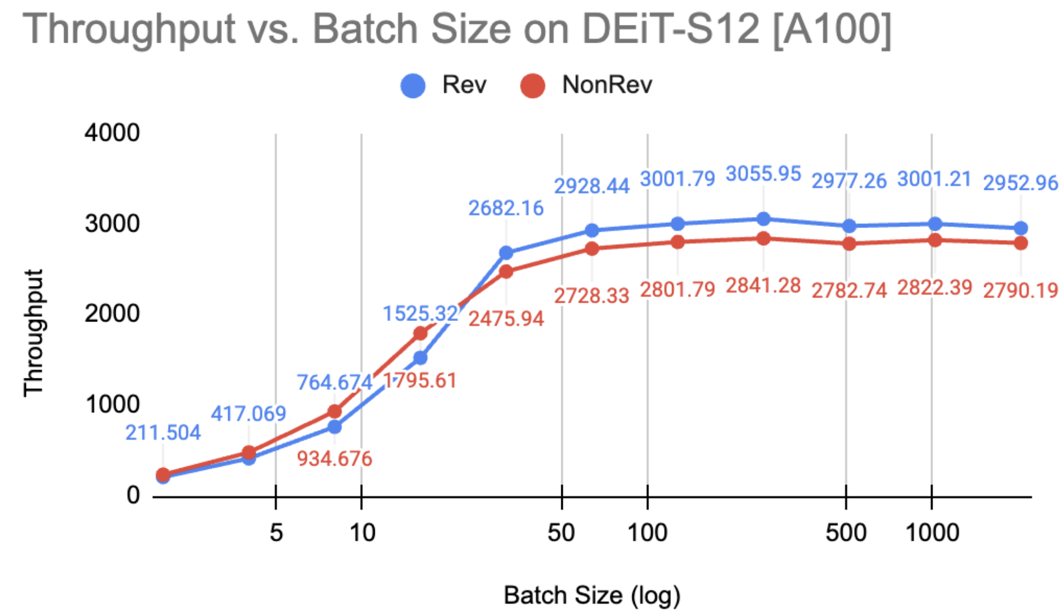
Example of the compute-bound roofline hitting around 64-128 batch size for a ViT-Small, from an old project of mine
Now let’s say you’ve been extra nice year so Santa dropped off a whole node of 8 GPUs. How can we speed up our model using more GPUs?
DDP: Suffering from Success
The key goal is to keep the GPUs warm as long as possible. In our case, our models fit on one GPU, so we’ll duplicate copies of our model across each device. Data remains the main knob we control. A good rule of thumb is to parallelize only when and what is necessary (we’ll quantify this later).
In effect, what we’re doing is running our model with a much larger batch size, split over all of the devices. This requires us to now manage the following:
- Distributing the data among all of the devices and running a forward pass
- Computing the gradients from each device on their specific mini-batch
- Synchronizing the gradients across all devices for backpropagation
This scheme is called Distributed Data Parallel, or DDP, as we parallelize our data and nothing else. We shard (split) our data across devices, and the only thing we need to manage are the gradients.
![DDP illustration, taken from [3].](https://blog.tylerzhu.com/images/fsdp-for-dummies/ddp_illustration.png)
DDP illustration, taken from [3].
Note that we don’t need to sync beyond the gradients. From the optimizer’s perspective, it’s simply optimizing a local model. Each replica starts from the same state and gets the same averaged gradients, so they naturally stay in sync [4].
How does this happen mechanically? This is powered by communication primitives which are the backbone of distributed programming. In our case, we want to combine (i.e. reductions like sum, min, avg) data across devices and store that result on each device, specifically the gradients. This is an all_reduce operation: it reduces data across all of the devices.
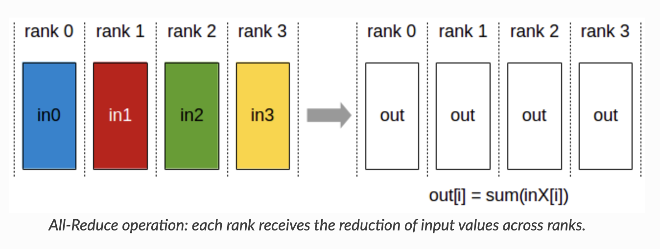
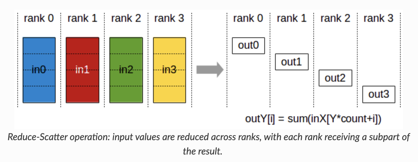
The all_reduce is actually a combination of two other primitives: the reduction step, and the gathering step. The first is a reduce_scatter, which reduces across all devices and scatters the result in equal-sized blocks across devices. You may wonder, why do we bother scattering after reducing? The answer is to reduce the amount of communication of course (and avoid unnecessary data transfer)!
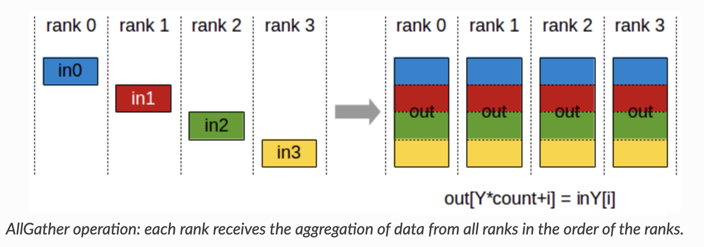
The second is the all_gather, which gathers scattered results across devices into each device. Visually it should be quite clear now why all_reduce = reduce_scatter -> all_gather. And that’s DDP in a nutshell!
What is the tradeoff now compared to the 1 GPU setting? Now we have to worry about communication costs for the gradients. Typically GPU<->GPU transfer is supported by NVLink, but my L40 GPUs don’t support it, so we’re still using the PCIe 4.0 x16 bus at 32 GB/s per direction speeds (10-20x slower than NVLink :|). In our case training small models, this isn’t much of an issue yet, but this can be prohibitive for 7B parameter LLMs (14GB of gradients -> 0.2-0.4s per step!).
In summary, we perform the following:
- Forward pass (local)
- Backward pass (local)
- All-reduce: Gradients are synchronized across GPUs
- Optimizer step (local, using synchronized gradients) Tradeoff: Somewhat redundant memory usage for storing copies of the model.
Some low-level details
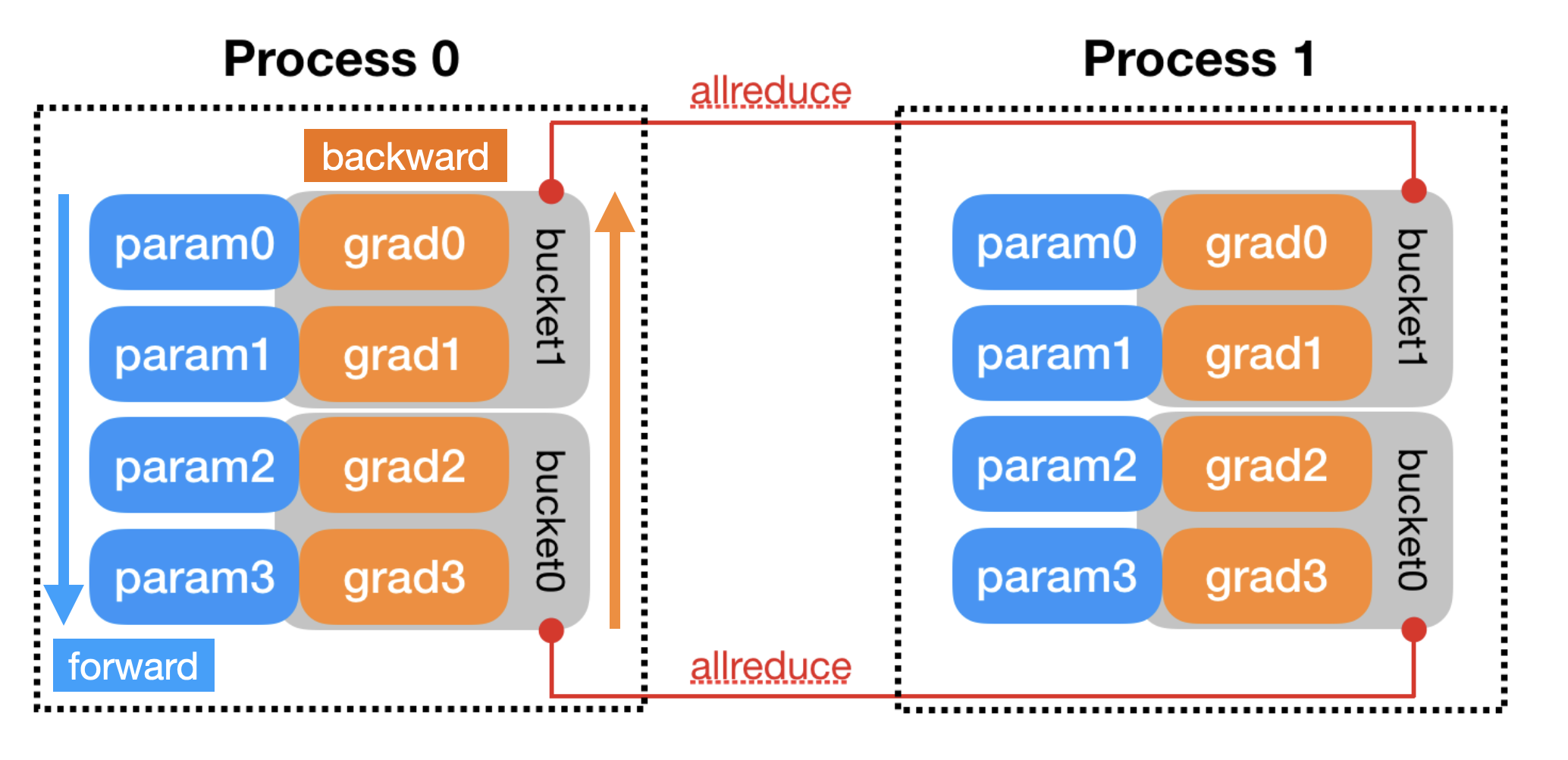
Reading [4] sheds some light on low-level implementation details of DDP. One is the practical issue of determining when to trigger an all_reduce, i.e. knowing when all devices are done computing a specific gradient so we can sync. This is done with backward hooks (since backward() is out of DDP’s control).
When one gradient is ready, its corresponding DDP hook on that grad accumulator will fire, and DDP will mark that parameter gradient as ready for reduction. … When all [gradients] are ready, the Reducer will block waiting for all
all_reduceoperations to finish. When this is done, averaged gradients are written to theparam.gradfield of all parameters. So after the backward pass, the grad field on the same corresponding parameter across different DDP processes should be the same.
However, naively calling an all_reduce for every single parameter would be catastrophic for your latency because each call has overhead. There is a fixed GPU data transfer launch time (~20 µs) to initiative a kernel or copy operation, which means many small calls will incur high latency.
One natural optimization is bucketing. To minimize communication costs, we group our parameters into buckets which are sent together. The buckets are assigned in approximately reverse order of the model.parameters(), since DDP expects gradients to become ready during the backward pass in approximately that order. (Actually, in recent versions, DDP tracks the param order in the first pass, then rebuilds buckets optimally [3]). This lets DDP pipeline the communication, transferring gradients for the last layers while the earlier ones are calculating. All in all, our overall throughput shouldn’t take much of a hit compared to normal training, although in practice Nx devices will lead to ~(N-0.5)x speedups.
By default, PyTorch DDP uses a bucket size of 25MB. If your GPU is not hitting high utilization in the backward pass, it means you are latency bound, so it could be useful to set this limit higher to utilize more compute power.
FSDP: BIG models need BIG sharding
Ding dong, it’s Most Surely Language at your door. Now they’re asking you to train LLMs, which are huge parameter models that barely fit on one GPU. What do you do?
Let’s walk through the lifecycle of a step in the pipeline to see what’s needed now.
- Dataset: While the overall dataset is large, with prefetching we only ever need a couple of batches in memory at a time. So this is hardly a prohibitive factor. We’ll distribute the data, just as in DDP.
- Model weights: Now we need to shard our weights across our devices to make our model fit into memory. For example, we could have Layer 1 on GPU 0, Layer 2 on GPU 1, etc. No single GPU holds the full model. In practice it will be more granular than this though.
- Forward pass: Let’s say we’re at Layer 1. Each device needs to process it’s own mini-batch, but the weights for Layer 1 are sharded across all of the devices. Therefore:
- Each device will broadcast their shard of Layer 1 (i.e. an
all_gather) - Temporarily, every device holds the full weights for Layer 1, so they do a forward pass on their local data.
- Immediately afterwards, every device drops the full Layer 1 weights, keeping only their original shard.
- Each device will broadcast their shard of Layer 1 (i.e. an
- Backward pass: Just like the forward pass. To compute gradients for e.g. Layer 1, we need to recollect all shards of Layer 1, then compute the gradients before dropping the weights again.
- Gradient update: This is where we differ from DDP. Remember that each device has a local gradient for Layer 1 from its own mini-batch, so we first need to average our gradients over all mini-batches. However, now the weights are scattered across our devices, so we don’t want to synchronize all gradients to every device, just to where the corresponding shards live. In fact, we have a primitive just for this:
reduce_scatter!
In this way, we simply use each device as storage for the parameters, as GPU storage is much faster than loading from disk (CPU). We’re trading network bandwidth (sending the weights around constantly with all_gather) for memory capacity (storing a fraction of the model per device).
Compared to DDP, we incur an extra all_gather per parameter, but because we’ve reduced the memory needed, we might be able to run with a larger batch size and still be faster.
The following summary from Tim Darcet distills this very clearly:
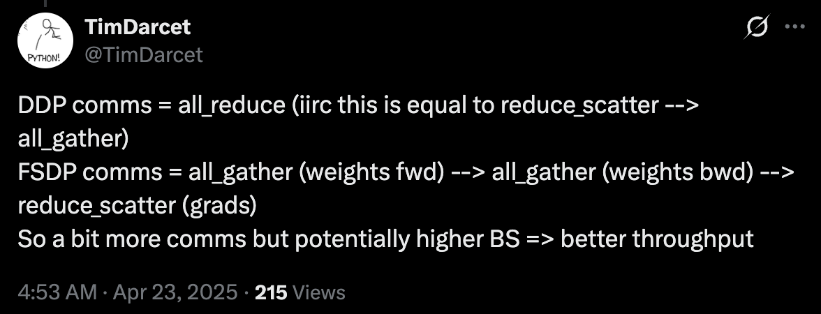
Tim Darcet’s summary of FSDP vs DDP
Deeper Details
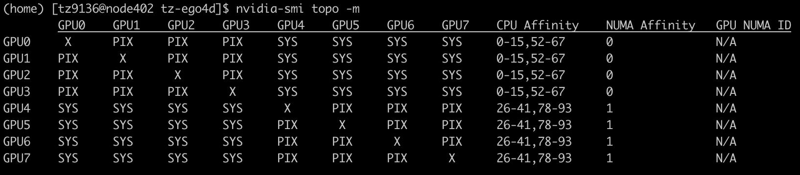
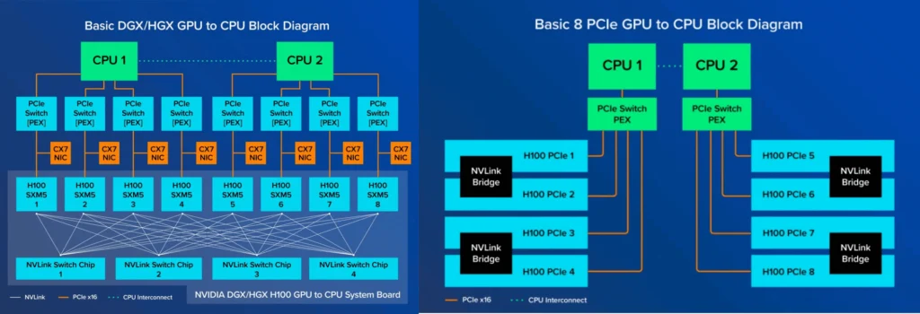
I actually looked at the topology of the GPUs I use using nvidia-smi topo -m. It checks out with the spec, and offers some additional details which are interesting.
Each cluster node is a Lenovo ThinkSystem SR670 V2 containing:
- 2 x Intel Xeon Gold 5320 26-core CPUs
- 16 x 32GB DDR4 3200MHz RDIMMs (512GB total)
- 8 x NVidia L40 GPUs
- 3.5TB of SSD for local scratch
- One 10Gbps Ethernet uplink (Note: NOT Infiniband)
So this makes sense, since each CPU is connected to 4 GPUs. The GPUs within each group have fast interconnect, while the GPUs across groups have slightly slower interconnect.
References
- https://x.com/TimDarcet/status/1914965730488955334
- https://horace.io/brrr_intro.html
- https://www.youtube.com/watch?v=RQfK_ViGzH0
- https://docs.pytorch.org/docs/main/notes/ddp.html
- https://dev-discuss.pytorch.org/t/fsdp-cudacachingallocator-an-outsider-newb-perspective/1486
- CAPI implementation of SimpleFSDP: https://github.com/facebookresearch/capi/blob/main/fsdp.py
- SimpleFSDP: https://arxiv.org/abs/2411.00284